1.　Introduction

Collaborative learning is a methodology that involves teaching and learning in groups of learners working together for problem-solving. Collaboration leads learners to integrate new ideas from other learners and enhance their social abilities through interaction with other learners. Researchers in learning science have qualitatively analyzed collaborative learning and revealed various patterns to increase learning performance [2], [12], [15], [16], [29], [30], [37], [42]. For example, the study in [29] found that learners using identical problem-solving methods tend to consistently produce higher learning outcomes. Through the process of collaborative learning analysis, transcription is an essential step for accurate analysis of collaboration. However, the transcription process was costly both financially and in human time because the researchers were forced to repeatedly watch the recorded video of collaborative learning and record the speech timing.

Speaker identification is a possible solution for reducing transcription difficulties. While most studies identify a speaker with audio data sampled at 8 kHz or more in the field of speaker recognition [1], [4]-[7], [25], [27], [28], [34], [44], several studies contribute to speaker identification with lower-sampled sound pressure acquired from IoT sensors for collaborative learning analysis [48]-[51]. Lower-sampled sound pressure is processable even in IoT sensors which mount a small and low-spec microcontroller owing to the small size. However, the studies are hampered by the situation that multiple users simultaneously speak such as speech overlap in turn-taking [12], [16], [42]. Such oversight causes inaccurate results of collaborative learning analysis.

Recent work has however demonstrated that a single speaker is accurately identified with lower-sampled sound pressure acquired from IoT sensors called Sensor-based Regulation Profiler Badges (SRP Badges) [51]. The study accurately distinguishes speech from the owner or other users with speech threshold in an environment with a single speaker at most. A question therefore is why not just replicate the threshold-based speaker identification to distinguish multiple speakers and non-speakers? There is an issue to apply the threshold-based speaker identification to an environment with multiple speakers.

The issue is exclusion of k out of n ($1 \leq k < n$) speakers as noise. The study in [51] regards a user whose detected speech is the longest as a speaker in each speech-estimated section. If the study encounters the situation that k out of n multiple users simultaneously speak, the detected speech of speakers will stretch in each section. However, the algorithm extracts only a user whose detected speech is the longest as a speaker in each section. The algorithm finally ignores other speakers while their detected speech is relatively long.

To solve the above issue, this paper proposes a novel multi-speaker identification algorithm for SRP Badges. The algorithm: 1) detects speech sections where at least one user speaks, 2) judges all users' speech in each speech section, and 3) divides speakers and non-speakers in each speech section whenever the second step does not judge all users' speech. The three steps algorithm accurately identifies multiple speakers with three-step speaker identification to clearly distinguish speakers and non-speakers. Experimental evaluations show that the algorithm follows the accuracy for single-speaker identification with SRP Badge [51] and accurately identifies multiple speakers with SRP Badge under different numbers of users, environmental noise, and users' short utterances.

This study has the following major contributions to the literature:

• ・Our research is the first study on simultaneous multi-speaker identification using mobile devices with low price and low power consumption.
• ・The proposed algorithm clearly distinguishes speakers and non-speakers based on the differences in sound pressure acquired from IoT sensors. The algorithm consists of three steps for speaker identification: speech section estimation, all-speakers judgment, and speaker identification.
• ・We quantitatively show the validity of our proposed speaker identification with experimental evaluations. Experimental evaluations show that the algorithm follows single-speaker identification with the IoT sensors [51] and accurately identifies multiple speakers with the IoT sensors in situations where there are different numbers of users, environmental noise, and users' short utterances.

The remainder of this paper is organized as follows: Section 2 describes related works. Section 3 presents the proposed algorithm for multiple-speaker identification. Experimental evaluations are conducted in Section 4. Section 5 finally concludes this paper.

2.　Related Works

This study is related to studies on speaker diarization and speaker recognition.

2.1　Speaker Diarization

Studies on speaker diarization [11], [13], [14], [19], [22]-[24], [32], [39], [40], [45], [47], [54]-[56] annotates audio with speaker labels by estimating how many users speak and assigning speech segments to each speaker. Speaker diarization has been applied to a variety of domains, such as telephone conversations [20], broadcast news [18], and meetings [10]. For example, the study in [10] proposes different architectures for information bottleneck-based diarization systems focusing on segment initialization and speaker discriminative representation and achieves a significant absolute improvement on standard meeting datasets. While those studies detect multiple speakers with recorded voices sampled at the high frequency of several kHz or more, this study identifies multiple speakers with sound pressure sampled at 100 Hz. Lower-sampled sound pressure is processable even in IoT sensors which mount a small and low-spec microcontroller owing to the small size.

2.2　Speaker Recognition

Speaker recognition refers to two different tasks: speaker verification and speaker identification. Studies on speaker verification [3], [8], [26], [31], [35], [41], [53] compare the voice of a speaker with that of a pre-registered person for authentication. Speaker verification is used for Internet of things (IoT) device authentication [38], network security [46], and user authentication [52]. For example, the study in [8] combines mel-frequency cepstral coefficients (MFCC) and linear predictive coding (LPC) to improve the performance of speaker verification for low-quality input speech signals. Studies on speaker identification [1], [4]-[7], [25], [27], [28], [34], [44] determine the speaker by comparing the voice of each speaker with the voice of a pre-registered person. Speaker identification has been applied to video conferences [43], criminal investigations [17], and television programs [33]. For example, the study in [43] proposes a method for robust speaker identification by focusing on a dominant speaker in a video conference, partially discarding information arising from inactive participants, and reducing the interference coming from their temporary speech.

While the above studies verify or identify a speaker with audio data sampled at 8 kHz or more, some studies [21], [48]-[51] identify a speaker with lower-sampled sound pressure acquired by IoT sensors. Lower-sampled sound pressure is processable even in IoT sensors that mount a small and low-spec microcontroller owing to the small size. For example, Rhythm [21] develops a business-card-type sensor called Rhythm Badge for speaker identification. Rhythm Badge consumes less power since it samples sound pressure at 700 Hz. Sensor-based Regulation Profiler (SRP) [49], [51] identifies a speaker with a novel algorithm for a business-card-type sensor called Sensor-based Regulation Profiler Badge (SRP Badge) to support collaborative learning analysis. The study in [49] showed SRP reduced analysis costs of collaborative learning in actual learning environments partly owing to speaker identification [51]. The SRP Badge mounts a peak-hold circuit to accurately detect the speech section and an RF module to synchronize across the sensors. SRP identifies a speaker more accurately than Rhythm using a sound pressure sampled at 100 Hz. However, the studies do not identify multiple speakers simultaneously. We propose a novel speaker identification algorithm for the SRP Badge [51] to simultaneously detect multiple speakers. The proposed algorithm accurately identifies multiple speakers who simultaneously speak with three steps 1) speech section estimation, 2) all-speakers judgment, and 3) speaker identification. Our experiments demonstrate that these three steps improve the accuracy of speaker identification for simultaneous speech.

3.　Proposed System: Speaker Identification

3.1　Overview

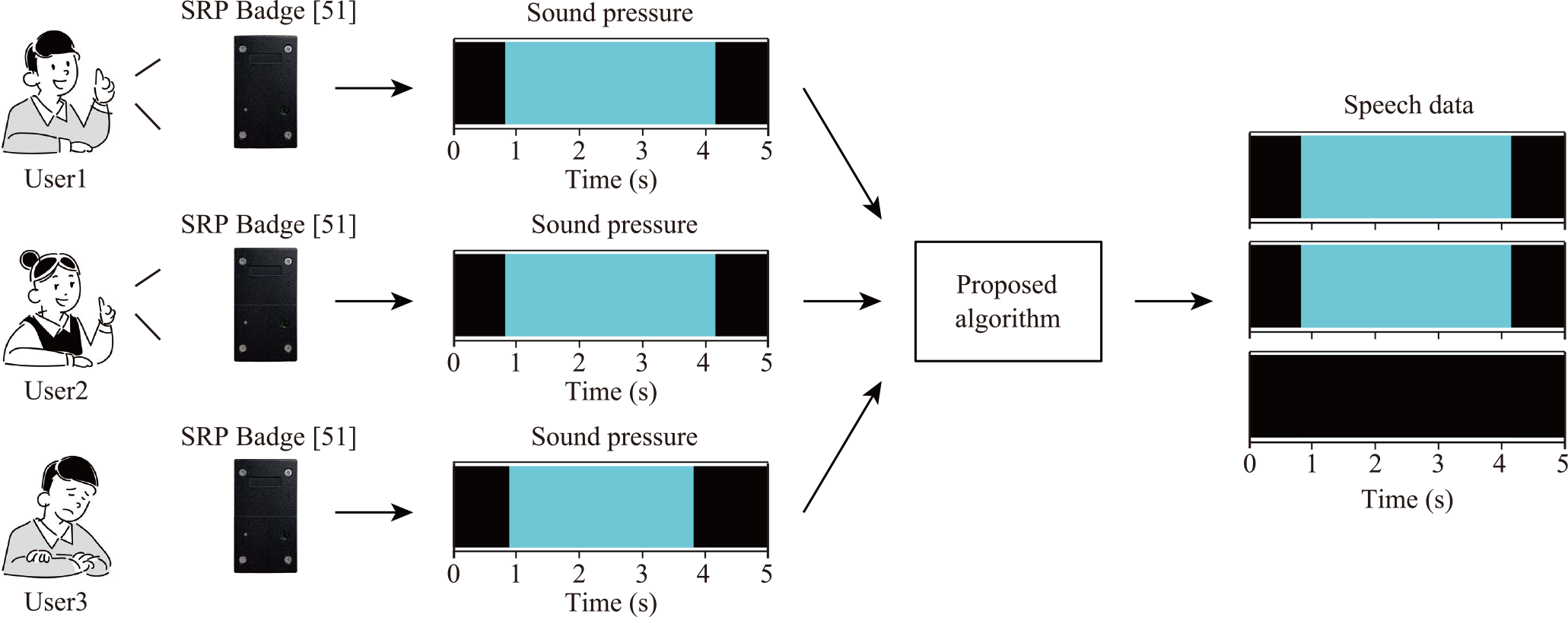
Figure 2 shows an overview of multi-speaker identification with the proposed algorithm. We include an IoT badge named Sensor-based Regulation Profiler Badge (SRP Badge) [51] to identify speakers with sound pressure data. SRP Badge is an IoT badge to be worn on the chest of each learner. SRP Badge mounts an accelerometer, an infrared sensor, and a sound pressure sensor. The badge can continuously run for 24 hours with a lithium-ion battery. INMP510 analog microphone from TDK is used as the sound pressure sensor for our proposed algorithm. INMP510 has a frequency response from 60 Hz to 20000 Hz in the conditions from low to high frequency −3 dB point. SRP Badge finally records only sound pressure at 100 Hz from the acquired voice with INMP510. In addition, SRP Badge precisely synchronizes the sound pressure data with other SRP Badges owing to a wireless synchronization module. We employ the following steps to identify the speakers with sound pressure data acquired from SRP Badges as shown in Fig. 2.

• (1)Distribute SRP Badges to learners before a collaborative learning activity
• (2)Acquire sound pressure signals from the learners with the SRP Badges during the learning activity
• (3)Collect the SRP Badges from the learners
• (4)Extract the sound pressure signals from the collected SRP Badges
• (5)Feed the sound pressure signals into the proposed speaker identification algorithm
• (6)Display the identification results with the proposed algorithms
• (7)Transcribe the learning activity with the identification results
• (8)Analyze the learning activity with the transcription results

3.2　Speaker Identification Algorithm

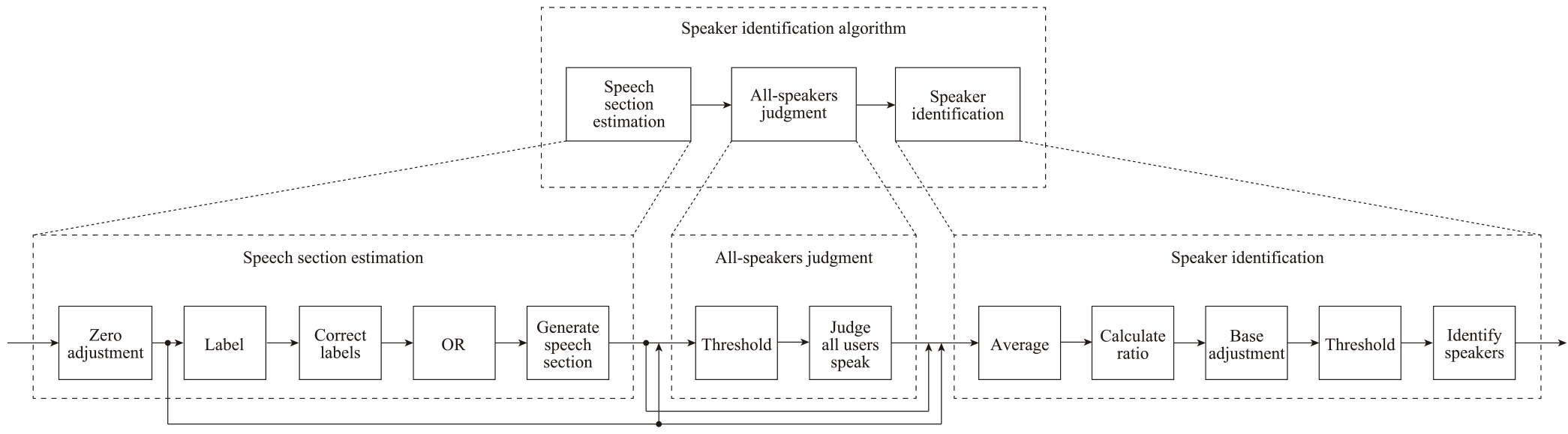
Figure 3 shows an overview of the proposed speaker identification algorithm. The algorithm consists of three steps: 1) speech section estimation, 2) all-speakers judgment, and 3) speaker identification.

Speech Section Estimation

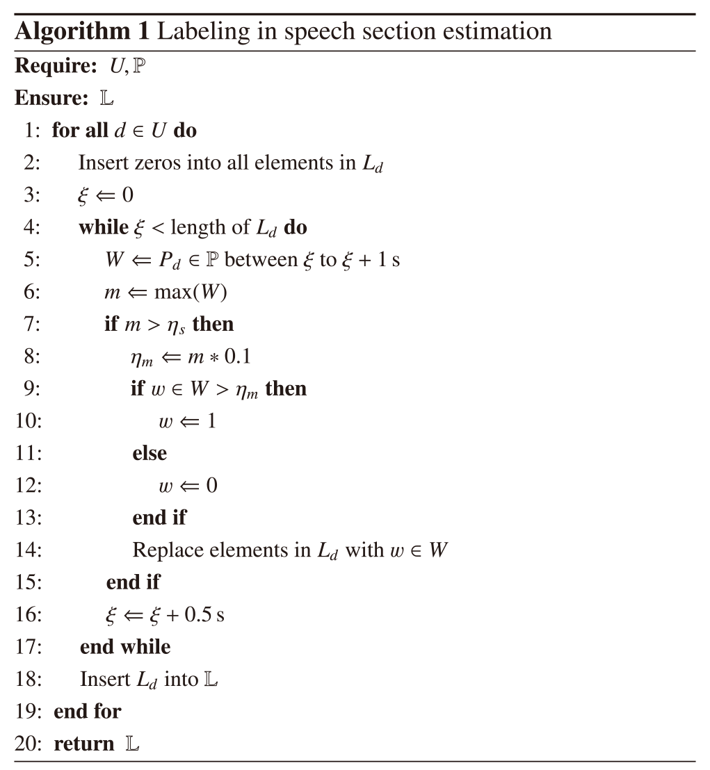
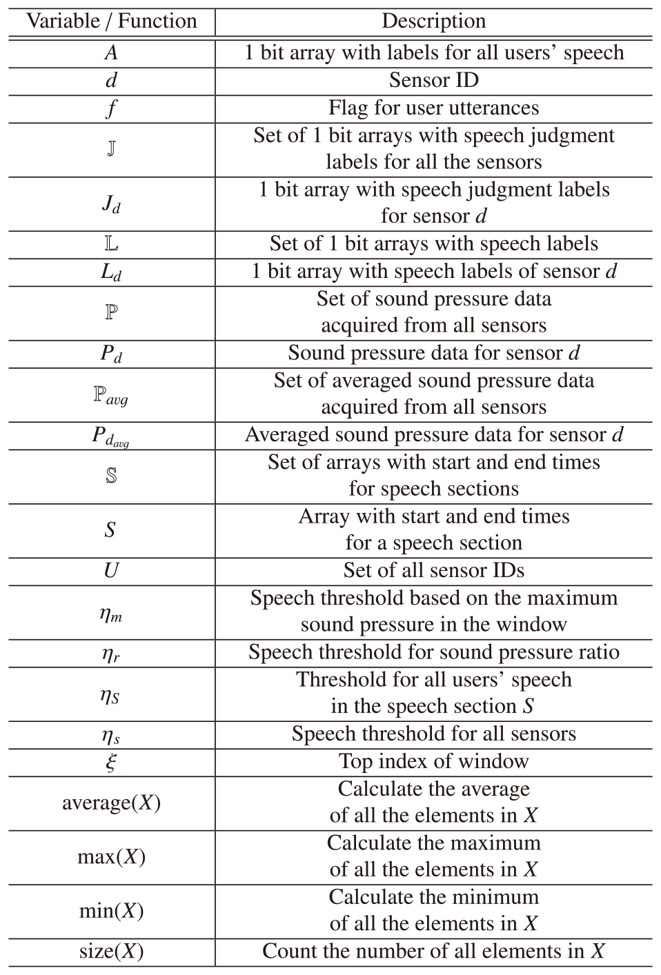
The first step estimates the presence or absence of users' speech from the acquired sound pressure signals for all the users' sensors. The algorithm finds the minimum value of sound pressure for all sensors and subtracts the minimum value from each value of sound pressure as a zero-point correction. The algorithm then labels whether more than one user is speaking using sliding windows for the sound pressure of each user acquired from the zero-point correction for each window. Algorithm 1 shows the process of labeling in Figure 3, and Table 1 lists the notation of the algorithm. The labeling algorithm outputs the array $\mathbb{L}$ representing “the 1–0 data for each user” from the set of all sensor IDs U and the set of the sound pressure data from all the sensors $ \mathbb{P} = \{ P_1,P_2, {\cdots} ,P_{|U|}\} $. Each window W finds the maximum value of sound pressure m for each sensor in line6. If the maximum value m in window W does not exceed the speech threshold $ \eta_s $ in all sensors, the algorithm regards window W as no speech section across the users, and the window slides in line16. If the value m exceeds the speech threshold $ \eta_s $, the algorithm updates a threshold $ \eta_m $ as $m \ast 0.1$ in line8 based on the study in [51]. The algorithm compares each sound pressure in a sensor with the threshold $\eta_m$ and assigns labels 1 or 0 if the sound pressure is higher or lower than the threshold $\eta_m$ in lines 9–13. The algorithm finally replaces the corresponding element in array $ L_d $ with the label w in window W in line14. We call the data acquired from the above pre-processing “the 1–0 data for each user.”The speech labels for each sensor are corrected with the 1–0 data for each user. The algorithm fills labels 1 in a section with continuous labels 0 within 90 ms between labels 1 as the middle of a speech in the 1–0 data for each user. The algorithm then replaces continuous labels 1 within 150 ms with labels 0 in a section, assuming that the section includes false speech caused by ambient noise. The acquired labels for each user are logically summed each time and combined as scalar binary data. We finally extract the binary data acquired from the above speech section estimation named “the speech section data.”

All-Speakers Judgment

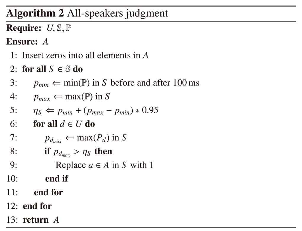
The second step judges whether all users are speaking in each speech section by combining the 1–0 data for each user and speech section data. The algorithm focuses on each section where a user is considered to speak based on the speech section data. Each speech section calculates the threshold based on the maximum and minimum sound pressure for all sensors and judges that all users are speaking if the sound pressure of all sensors exceeds the threshold. Algorithm 2 shows the procedure for all-speakers judgments in Figure 3, and Table 1 lists the notation of the algorithm. The judgment algorithm outputs the array A, which represents the result of all users' speech from the set of all sensor IDs U, the speech sections $\mathbb{S}$ extracted from 1) speech section estimation, and the set of the sound pressure data from all the sensors $ \mathbb{P} = \{ P_1,P_2, {\cdots} ,P_{|U|}\} $. The algorithm finds the minimum sound pressure $p_{min}$ from 100 ms before and after each speech section in all the sensors to estimate the noise floor in line3. Although the speech section is considered as enough to get the minimum sound pressure, we set the inclusive section with the margin of 100 ms to find the minimum in case. The algorithm also finds the maximum sound pressure $p_{max}$ from each speech section in all sensors in line4. Based on the values of $p_{min}$ and $p_{max}$, the algorithm sets the threshold for all users' speech $\eta_S$ as $p_{min} + (p_{max} - p_{min})\ast 0.95$ in line5. We chose the best parameter for the speech threshold $\eta_S$ as 0.95, which did not decrease the accuracy so much and would prevent the lenient judgment of all-users speech. If the speech section for all sensors exceeds the threshold $\eta_S$, the algorithm judges that all users are speaking in the speech section S and sets the label1 for all users' speech in section S in lines6–11. Finally, the algorithm returns the labels for all users' speech in the all-speech sections A.

Speaker Identification

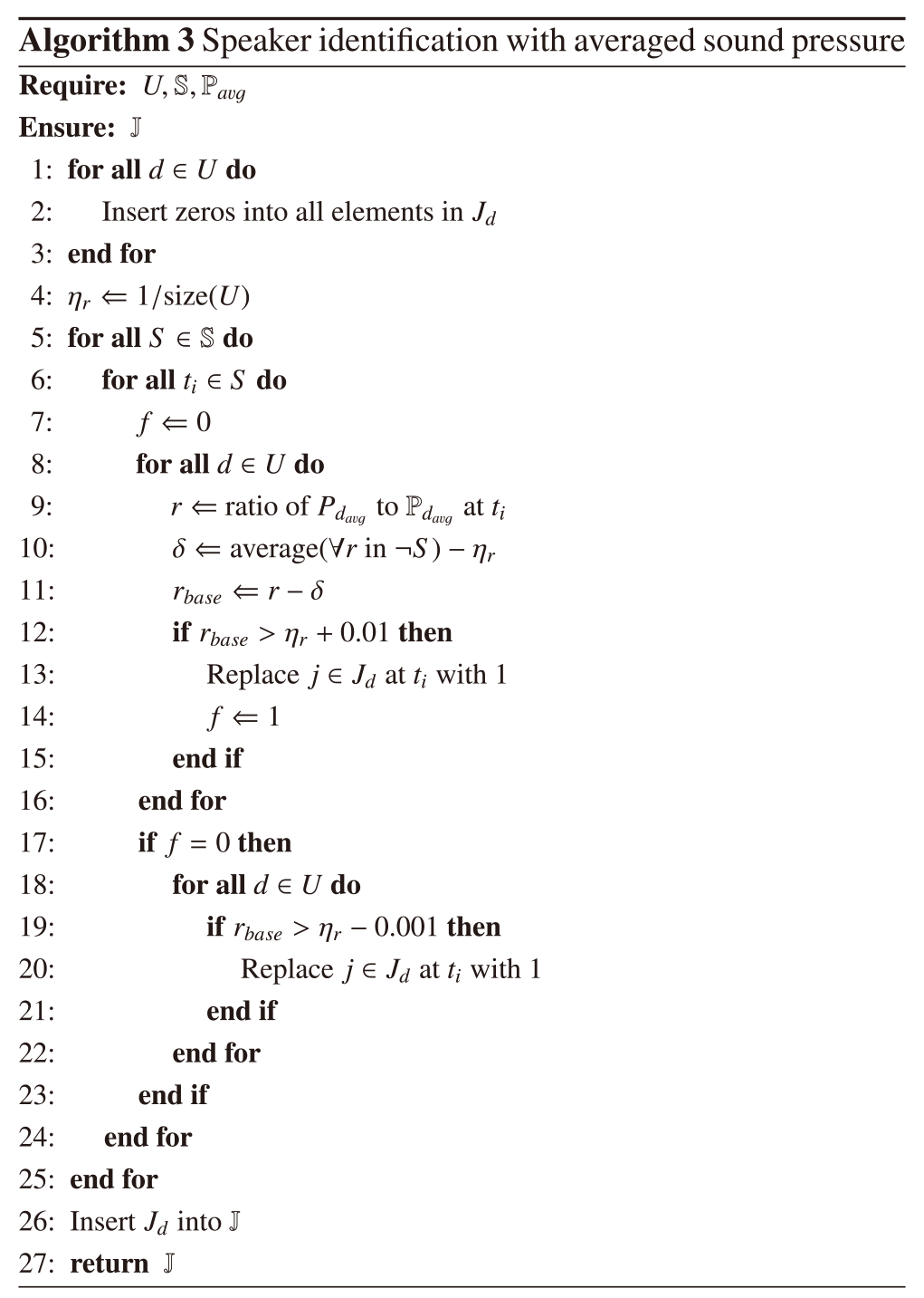
The third step determines who is speaking in each speech section using an averaged, relativized, and base-adjusted sound pressure. Each speech section estimates where a user speaks based on the speech section data. The algorithm judges each user's speech using the ratio of sound pressure compared to the speech threshold. The averaged sound pressure for each sensor is calculated using sliding windows with a window size of 0.5 s and a slide width of 0.01 s. We note that we set the window size and the slide width to finely extract changing simultaneous speech by multiple speakers. The algorithm identifies speakers with the averaged sound pressures for all users $\mathbb{P}_{avg}$. Algorithm 3 shows the procedure for speaker identification with averaged sound pressure in Figure 3, and Table 1 lists the notation of the algorithm. The identification algorithm outputs the array $\mathbb{J}$, which represents the judged speech labels for each user from the set of all sensor IDs U, the speech sections $\mathbb{S}$ extracted from 1) speech section estimation, and the averaged sound pressure data from all the sensors $\mathbb{P}_{avg} = \{ P_{1_{avg}},P_{2_{avg}}, {\cdots} ,P_{|U|_{avg}}\} $. The algorithm sets the speech threshold ${\eta_r}$ based on the number of sensors U in line4. The algorithm then calculates the sound pressure ratio of each sensor for all sensors r based on the averaged sound pressure for each sensor $p \in P_{d_{avg}}$ at each time ${t_i}$ in the speech section $S \in \mathbb{S}$ in line 9. The offset in each sensor $ \delta $ is calculated based on the difference between the averaged sound pressure ratio of each sensor in all non-speech sections $\neg S$ and the speech threshold $ \eta_r $ as a base adjustment in line10. The algorithm subtracts the offset in each sensor $ \delta $ from the sound pressure ratio of each sensor r in line11. The algorithm then judges multiple speakers in each speech section $ S \in \mathbb{S} $ using a two-step speaker identification with the averaged and base-adjusted ratio $r_{base}$. If the ratio $r_{base}$ for sensor d exceeds the summation of the threshold $\eta_r$ and the allowable error 0.01 in the speech section S, the first algorithm judges that the user with sensor d speaks in section S in lines12–15. The first judgment detects clear speech with only a few people speaking. We chose the best parameter for the threshold $\eta_r$ as 0.01, which did not decrease the accuracy so much and would prevent the judgment of noise as speech. If the first algorithm judges that no one is speaking in the speech section S, the second algorithm judges multiple speakers in the same way as the first judgment with an allowable error of −0.001 in section S in lines18–22. The second judgment detects ambiguous speech with many people speaking. We experimentally chose the parameter as 0.001 to set the threshold lower than the first threshold not to miss the ambiguous speech. Finally, the algorithm returns the speech labels for each sensor $\mathbb{J}$.

4.　Evaluation: Speaker Identification Accuracy

We experimentally evaluated the accuracy of the proposed algorithm for detecting simultaneous speech using sound pressure data acquired from SRP Badges. We experimented in a conference room considering varying numbers of users, environmental noises, and users' short utterances. We note that our study supposes a situation under environmental noises from video material [9] learners play in collaborative learning activities. Subjects were male university students in their early 20 s. Each dimension of the room was 10.6 m, 7.05 m, and 2.65 m, respectively. We considered the influence of reverberation in the room supposed to be used in collaborative learning. Each user wore SRP Badge on his chest and sat on a chair 1.50 m away from adjacent users. We set a synchronizer on a table at the center of the users for time synchronization between the sensors. For the experiments with long and short utterances, we prepared two types of speech scripts for each user [51]. Each script included 15 sentences in English. Specifically, all users spoke a sentence in the script in order with a two-second interval. After all the users spoke a sentence, the users started to speak the next sentence. We changed all combinations of users who simultaneously spoke in each sentence. For example, when there are three users in an experiment, the combinations are as follows:

• ・One user speaks, and the two others do not speak
• ・Two users simultaneously speak and the other does not speak
• ・Three users simultaneously speak

In each case, we changed all combinations of speakers and non-speakers by considering the difference in users' voice characteristics.

We compared the speaker identification accuracy of our proposed scheme with three comparison schemes, “Scheme with absolute sound pressure (absolute scheme),” “Scheme with relative sound pressure (relative scheme),” and “Extended scheme of the study in [21] (Rhythm scheme).” The absolute and relative schemes adopt speech-section estimation from part of the proposed algorithm in Sec. 3.2. The absolute scheme identified multiple speakers with a speech threshold for each speech section in a similar way to 2) all-speakers judgment in Sec. 3.2. The scheme calculated the threshold $\eta_S$ in each speech section S for each user and identified each user's speech. The relative scheme identified multiple speakers with the averaged and base-adjusted sound pressure and thresholding in the same way as 3) speaker identification in Sec. 3.2. The optimal threshold of speech detection for both algorithms depended on each evaluation setting. The Rhythm scheme was based on the study of [21] to identify a speaker with IoT badges named Rhythm Badge. We extended the study of [21] to identify multiple speakers. The original scheme in Rhythm applied the VAD algorithm [36] and the thresholding algorithm to single-speaker identification for human organization management. The VAD algorithm used sliding windows for the acquired power of sound pressure to reduce noise. The thresholding algorithm identified a user whose detected speech section was the longest as a speaker in each speech section. We extended the thresholding algorithm to simultaneously detect multiple speakers by judging speech for each user. We set the window size and the slide width to 2 s and 0.01 s for the sliding window in the VAD algorithm based on the study in [51]. The optimal value of the speech detection threshold for the thresholding algorithm depended on the evaluation settings.

4.1　The Number of Users

We show the speaker identification accuracy considering different numbers of users with a script of long speech utterances. The number of users varied from two to five. We set the speech threshold $\eta_s$ of Algorithm 1 in the absolute, relative, and proposed algorithm to 75 dB for the speech section estimation referring to the study in [51]. We also set the speech threshold in the Rhythm scheme to 84 dB for the speech estimation referring to the study in [51]. The threshold was appropriately met irrespective of the number of users.

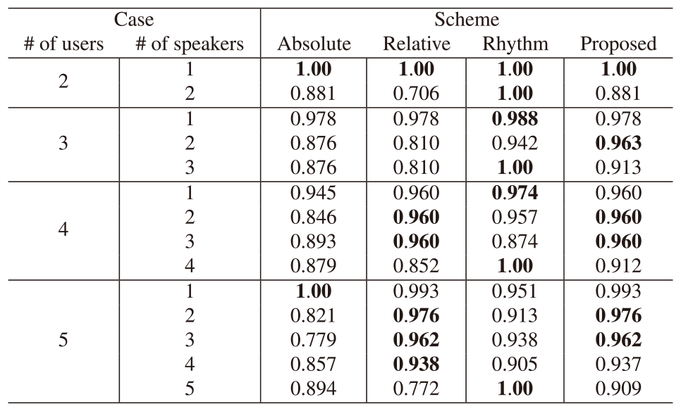
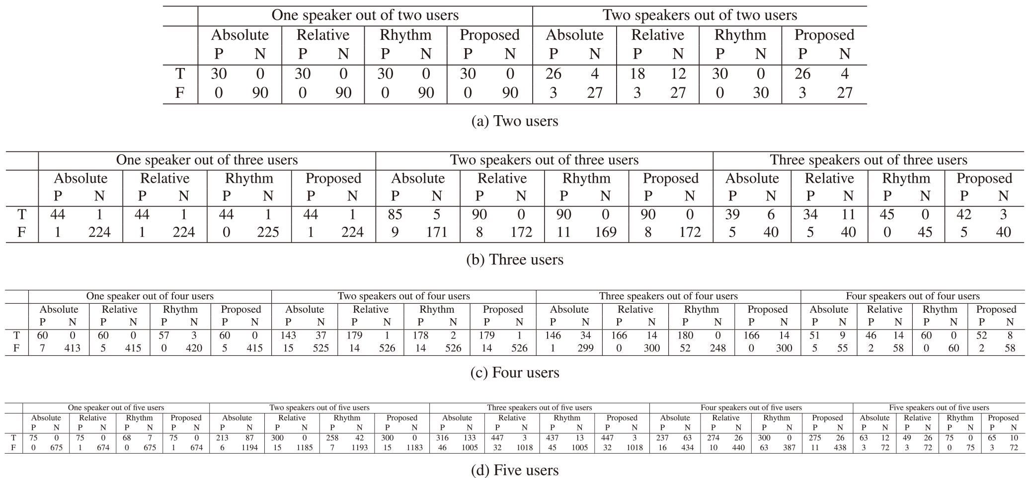
Tables 2 and 3 show the F1-scores of each scheme and the corresponding confusion matrices for two through five users. Each symbol on Table 3 shows that there was a speech (T) or not (F) and the proposed algorithm estimated speech (P) or non-speech (N). Compared with the absolute and relative schemes, the proposed scheme absorbed the advantages of each comparative scheme. The proposed algorithm precisely detected speakers in all-speakers cases with a combination of the two comparative schemes. As for the detection of the middle number of speech, the proposed scheme achieved high F1-scores taking advantage of the relative scheme. The proposed scheme also detected a single speaker with the advantage of the two comparative schemes in most cases. Table 3 indicated that two F1-scores of the proposed scheme were slightly lower than those of the two comparative schemes in the cases of 1 and 4 speakers out of 5 users since the threshold mistakenly regarded a non-speaker as a speaker (False Positive). Compared with the Rhythm scheme, the proposed scheme precisely detected the middle number of speakers such as 2 speakers out of 3 users, 2 and 3 speakers out of 4 users, 2, 3, and 4 speakers out of 4 users, and 2, 3, 4, and 5 speakers out of 5 users. Table 3 indicated that our proposed scheme accurately avoided falsely regarding non-speakers as speakers (False Positive) in most cases.

4.2　Environmental Noise

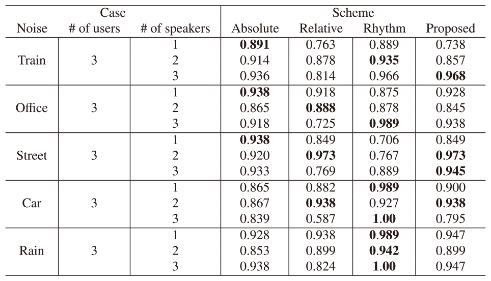
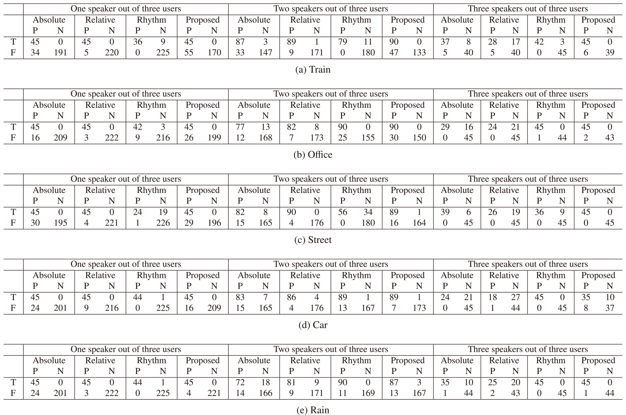
We show the influence of environmental noise on speaker identification accuracy. Three users participated in the experiments. We prepared a source to generate noise in our environment. The ceiling of the room furnished the noise source, 2 m, away from the table. The noise source generated five types of ambient noise recorded in trains, offices, streets, cars, and rain. Other settings were the same as the experiments in Sec.4.1. We set each noise as 75 dB in the train, 70 dB in the office and street, and 60 dB for cars and rain on average. We set the speech thresholds $\eta_s$ of Algorithm 1 in the absolute, relative, and proposed algorithm to 84 dB, 85 dB, 84 dB, 83 dB, and 80 dB for train, office, street, car, and rain noises for speech section estimation referring to the study in [51]. We also set the speech threshold in the Rhythm scheme to 89 dB, 86 dB, 89 dB, 84 dB, and 85 dB for train, office, street, car, and rain noises for the speech estimation referring to the study in [51].

Tables 4 and 5 show the F1-scores of each scheme and the corresponding confusion matrices under different environmental noises. Each symbol on Table 5 shows that there was a speech (T) or not (F) and the proposed algorithm estimated speech (P) or non-speech (N). Compared with the absolute and relative schemes, the proposed scheme precisely detected speakers without some cases absorbing advantages of the two comparative schemes. Table 3 indicated that F1-scores of the proposed scheme were slightly lower than those of the two comparative schemes in the cases of 1 and 2 speakers out of 3 users in the train, 1 and 2 speakers out of 3 users in the office, 1 speaker out of 3 users on the street, and 3 speakers out of 3 users in the car since the threshold mistakenly regarded a non-speaker as a speaker (False Positive). Compared with the Rhythm scheme, the proposed scheme precisely detected speakers under specific noise such as street. However, Table 4 indicated that the Rhythm scheme achieved precise speaker identification under the noise of rain. In terms of the frequency component in the noise, the noise of street included much frequency component between 10 Hz and 20 Hz, less than the Nyquist frequency of the sound pressure sensor in SRP Badge. We found that the proposed scheme had tolerance for low-frequency noise. On the other hand, the noise of rain entirely included noise in the frequency between 0 Hz and 50 Hz. We found that the proposed scheme had limitations of the above uniform noise.

4.3　Short Utterances

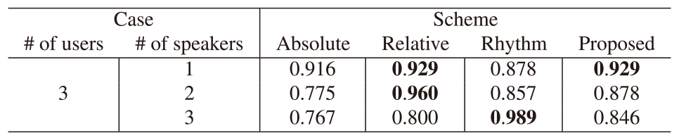
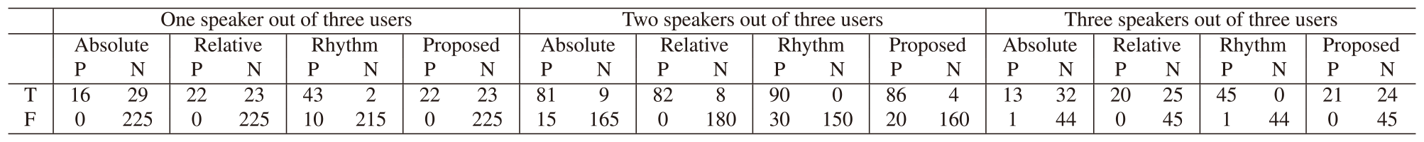
We show the influence of short utterances and speeches of less than one second [4], using the script of short utterances in the speech script. The experiments were conducted on three users. Other settings were the same as the experiments in Sec. 4.1. We set the speech threshold $\eta_s$ of Algorithm 1 in the absolute, relative, and proposed algorithm to 73 dB for speech section estimation referring to the study in [51]. We also set the speech threshold in the Rhythm scheme to 78 dB for the speech estimation referring to the study in [51].

Tables 6 and 7 show the F1-scores of each scheme and the corresponding confusion matrices of short utterances. Each symbol on Table 7 shows that there was a speech (T) or not (F) and the proposed algorithm estimated speech (P) or non-speech (N). Compared with the absolute and relative schemes, the proposed scheme absorbed the advantages of each comparative scheme. The proposed scheme precisely detected three speakers with the advantage of the absolute scheme. As for the single-speaker detection, the proposed algorithm achieved high F1-scores taking advantage of the relative scheme. Table 7 indicated that the F1-score of the proposed scheme was slightly lower than the relative scheme in the case of 2 speakers out of 3 users since the threshold mistakenly regarded a non-speaker as a speaker (False Positive). Compared with the Rhythm scheme, the proposed scheme precisely detected speakers in the cases of 1 and 2 speakers out of 3 users. Table 7 indicated that the F1-score of the proposed scheme was slightly lower than that of the Rhythm scheme in the all-speakers case since the threshold mistakenly regarded a speaker as a non-speaker (True Negative).

5.　Conclusion

In this study, we proposed a novel algorithm for multi-speaker identification with business-card-type sensors to extract collaboration characteristics in multi-person activities. The proposed algorithm simultaneously identifies multiple speakers using low-cost sensors through three steps: speech section estimation, all-speakers' judgment, and speaker identification. The steps eliminate ambient noise from non-speakers sensors to simultaneously identify multiple speakers with high accuracy. The evaluations showed that the algorithm accurately identified multiple speakers in a multi-person activity under different numbers of users, environmental noises, and users' short utterances.

For our future works, we plan to validate the specification of our proposed scheme, further justify the evaluation, and improve the accuracy of our proposed scheme under specific environments. We attempt to validate the influence of directivity in SRP Badge and the effect of reverberation in our proposed scheme. To further justify the evaluation, we plan to add experimental samples with various subjects and test significant differences between each scheme. We also attempt to precisely tune parameters in our proposed algorithm or acquire audio data from SRP Badge keeping low costs of hardware and processing to improve the accuracy of multi-speaker identification under specific environments.

Acknowledgments　This work was supported by JSPS KAKENHI Grant Number JP19H01714, JP22J20391, and JST PRESTO Grant Number JPMJPR2032, Japan.

References

- [1] Ajgou, R., Sbaa, S., Ghendir, S., Chamsa, A. and Taleb-Ahmed, A.: Robust Remote Speaker Recognition System Based on AR-MFCC Features and Efficient Speech Activity Detection Algorithm, International Symposium on Wireless Communications Systems, pp.722–727 (2014).
- [2] Backer, L. D., Keer, H. V., Smedt, F. D., Merchie, E. and Valcke, M.: Identifying regulation profiles during computer-supported collaborative learning and examining their relation with students' performance, motivation, and self-efficacy for learning, Computers & Education, Vol.179, p.104421 (2022).
- [3] Belfield,W. and Mikkilineni, R.: Speaker Verification Based on a Vector Quantization Approach that Incorporates Speaker Cohort Models and a Linear Discriminator, IEEE International Conference on Systems, Man, and Cybernetics. Computational Cybernetics and Simulation, pp.4525–4529 (1997).
- [4] Biagetti, G., Crippa, P., Curzi, A., Orcioni, S. and Turchetti, C.: Speaker Identification with Short Sequences of Speech Frames, International Conference on Pattern Recognition Applications and Methods, pp.178–185 (2015).
- [5] Biagetti, G., Crippa, P., Falaschetti, L., Orcioni, S. and Turchetti, C.: Speaker Identification in Noisy Conditions Using Short Sequences of Speech Frames, Smart Innovation, Systems and Technologies, pp.43–52 (2018).
- [6] Brunet, K., Taam, K., Cherrier, E., Faye, N. and Rosenberger, C.: Speaker Recognition for Mobile User Authentication: An Android Solution, Conférence sur la Sécurité des Architectures Réseaux et Systèmes d'Information, pp.1–10 (2013).
- [7] Chakroborty, S., Roy, A. and Saha, G.: Fusion of a Complementary Feature Set with MFCC for Improved Closed Set Text-Independent Speaker Identification, IEEE International Conference on Industrial Technology, Vol.387–390 (2006).
- [8] Chowdhury, A. and Ross, A.: Fusing MFCC and LPC Features Using 1D Triplet CNN for Speaker Recognition in Severely Degraded Audio Signals, IEEE Transactions on Information Forensics and Security, Vol.15, pp.1616–1629 (2020).
- [9] Cognition and at Vanderbilt, T. G.: The Jasper Series as an Example of Anchored Instruction: Theory, Program Description, and Assessment Data, Educational Psychologist, Vol.27, No.3, pp.291–315 (1992).
- [10] Dawalatabad, N., Madikeri, S., Sekhar, C. C. and Murthy, H. A.: Novel Architectures for Unsupervised Information Bottleneck Based Speaker Diarization of Meetings, IEEE/ACM Transactions on Audio, Speech, and Language Processing, Vol.29, pp.14–27 (2021).
- [11] Dubey, H., Sangwan, A. and Hansen, J. H. L.: Transfer Learning Using Raw Waveform Sincnet for Robust Speaker Diarization, IEEE International Conference on Acoustics, Speech and Signal Processing, pp.6296–6300 (2019).
- [12] Evans, M. A., Feenstra, E., Ryon, E. and McNeill, D.: A multimodal approach to coding discourse: Collaboration, distributed cognition, and geometric reasoning, International Journal of Computer-Supported Collaborative Learning, Vol.6, pp.253–278 (2011).
- [13] Fujita, Y., Kanda, N., Horiguchi, S., Xue, Y., Nagamatsu, K. and Watanabe, S.: End-to-End Neural Speaker Diarization with Self-Attention, IEEE Automatic Speech Recognition and Understanding Workshop, pp.296–303 (2019).
- [14] Garcia-Romero, D., Snyder, D., Sell, G., Povey, D. and McCree, A.: Speaker Diarization using Deep Neural Network Embeddings, IEEE International Conference on Acoustics, Speech and Signal Processing, pp.4930–4934 (2017).
- [15] Haataja, E., Malmberg, J. and Järvelä, S.: Monitoring in collaborative learning: Co-occurrence of observed behavior and physiological synchrony explored, Computers in Human Behavior, Vol.87, pp.337–347 (2018).
- [16] Haller, C. R., Gallagher, V. J., Weldon, T. L. and Felder, R. M.: Dynamics of Peer Education in Cooperative Learning Workgroups, Journal of Engineering Education, Vol.89, No.3, pp.286–293 (2000).
- [17] Karadaghi, R., Hertlein, H. and Ariyaeeinia, A.: Effectiveness in Open-Set Speaker Identification, International Carnahan Conference on Security Technology, pp.1–6 (2014).
- [18] Lan, G. L., Charlet, D., Larcher, A. and Meignier, S.: Iterative PLDA Adaptation for Speaker Diarization, INTERSPEECH, pp.2175–2179 (2016).
- [19] Lan, G. L., Charlet, D., Larcher, A. and Meignier, S.: A Triplet Ranking-based Neural Network for Speaker Diarization and Linking, INTERSPEECH, pp.3572–3576 (2017).
- [20] Lapidot, I. and Bonastre, J.-F.: Integration of LDA into a Telephone Conversation Speaker Diarization System, IEEE Convention of Electrical and Electronics Engineers in Israel, pp.1–4 (2012).
- [21] Lederman, O., Mohan, A., Calacci, D. and Pentland, A. S.: Rhythm: A Unified Measurement Platform for Human Organizations, IEEE MultiMedia, Vol.25, No.1, pp.26–38 (2018).
- [22] Lin, Q., Yin, R., Li, M., Bredin, H. and Barras, C.: LSTM based Similarity Measurement with Spectral Clustering for Speaker Diarization, INTERSPEECH, pp.366–370 (2019).
- [23] Madikeri, S. and Bourlard, H.: Filterbank Slope based Features for Speaker Diarization, IEEE International Conference on Acoustics, Speech and Signal Processing, pp.111–115 (2014).
- [24] Madikeri, S., Motlicek, P. and Bourlard, H.: Combining SGMM Speaker Vectors and KL-HMM Approach for Speaker Diarization, IEEE International Conference on Acoustics, Speech and Signal Processing, pp.4834–4838 (2015).
- [25] Matsumoto, K., Hayasaka, N. and Iiguni, Y.: Noise Robust Speaker Identification by Dividing MFCC, International Symposium on Communications, Control and Signal Processing, pp.652–655 (2014).
- [26] Ming, J., Hazen, T. J., Glass, J. R. and Reynolds, D. A.: Robust Speaker Recognition in Noisy Conditions, IEEE Transactions on Audio, Speech, and Language Processing, Vol.15, No.5, pp.1711–1723 (2007).
- [27] Nakagawa, S., Wang, L. and Ohtsuka, S.: Speaker Identification and Verification by Combining MFCC and Phase Information, IEEE Transactions on Audio, Speech, and Language Processing, Vol.20, No.4, pp.1085–1095 (2012).
- [28] Nishimura, J. and Kuroda, T.: Hybrid Speaker Recognition Using Universal Acoustic Model, SICE Journal of Control, Measurement, and System Integration, Vol.4, No.6, pp.410–416 (2011).
- [29] Oshima, J., Oshima, R. and Fujii, K.: Student Regulation of Collaborative Learning in Multiple Document Integration, The Proceedings of the International Conference of the Learning Science (ICLS), Vol.2, pp.967–971 (2014).
- [30] Oshima, J., Oshima, R. and Fujita, W.: A Mixed-Methods Approach to Analyze Shared Epistemic Agency in Jigsaw Instruction at Multiple Scales of Temporality, Journal of Learning Analytics, Vol.5, No.1, pp.10–24 (2018).
- [31] Pandiaraj, S., Keziah, H. N. R., Vinothini, D. S., Gloria, L. and Kumar, K. R. S.: A Confidence Measure based ― Score Fusion Technique to Integrate MFCC and Pitch for Speaker Verification, International Conference on Electronics Computer Technology, pp.317–320 (2011).
- [32] Park, T. J., Han, K. J., Huang, J., He, X., Zhou, B., Georgiou, P. and Narayanan, S.: Speaker Diarization with Lexical Information, INTERSPEECH, Vol.391–395 (2019).
- [33] Poignant, J., Besacier, L. and Quénot, G.: Unsupervised Speaker Identification in TV Broadcast Based on Written Names, IEEE/ACM Transactions on Audio, Speech, and Language Processing, Vol.23, No.1, pp.57–68 (2015).
- [34] Reynolds, D. A.: Experimental Evaluation of Features for Robust Speaker Identification, IEEE Transactions on Speech and Audio Processing, Vol.2, No.4, pp.639–643 (1994).
- [35] Roy, A., Magimai.-Doss, M. and Marcel, S.: A Fast Parts-Based Approach to Speaker Verification Using Boosted Slice Classifiers, IEEE Transactions on Information Forensics and Security, Vol.7, No.1, pp.241–254 (2012).
- [36] Sangwan, A., Chiranth, M. C., Jamadagni, H. S., Sah, R., Prasad, R. V. and Gaurav, V.: VAD Techniques for Real-Time Speech Transmission on the Internet, IEEE International Conference on High Speed Networks and Multimedia Communication, pp.46–50 (2002).
- [37] Sawyer, R. K.: Cambridge Handbook of the Learning Sciences, Second Edition, Cambridge University Press (2014).
- [38] Shin, D.-G. and Jun, M.-S.: Home IoT Device Certification through Speaker Recognition, International Conference on Advanced Communication Technology, pp.600–603 (2015).
- [39] Shum, S., Dehak, N., Chuangsuwanich, E., Reynolds, D. and Glass, J.: Exploiting Intra-Conversation Variability for Speaker Diarization, INTERSPEECH, No.945–948 (2011).
- [40] Sun, G., Zhang, C. and Woodland, P. C.: Speaker Diarisation Using 2D Self-Attentive Combination of Embeddings, IEEE International Conference on Acoustics, Speech and Signal Processing, pp.5801–5805 (2019).
- [41] Taherian, H., Wang, Z.-Q., Chang, J. and Wang, D.: Robust Speaker Recognition Based on Single-Channel and Multi-Channel Speech Enhancement, IEEE/ACM Transactions on Audio, Speech, and Language Processing, Vol.28, pp.1293–1302 (2020).
- [42] Vass, E., Littleton, K., Miell, D. and Jones, A.: The discourse of collaborative creative writing: Peer collaboration as a context for mutual inspiration, Thinking Skills and Creativity, Vol.3, No.3, pp.192–202 (2008).
- [43] Volfin, I. and Cohen, I.: Dominant Speaker Identification for Multipoint Videoconferencing, IEEE Convention of Electrical and Electronics Engineers in Israel, pp.1–4 (2012).
- [44] Wali, S. S., Hatture, S. M. and Nandyal, S.: MFCC Based Text-Dependent Speaker Identification Using BPNN, International Journal of Signal Processing Systems, Vol.3, No.1, pp.30–34 (2015).
- [45] Wang, Q., Downey, C., Wan, L., Mansfield, P. A. and Moreno, I. L.: Speaker Diarization with LSTM, IEEE International Conference on Acoustics, Speech and Signal Processing, pp.5239–5243 (2018).
- [46] Wu, Z., Leon, P. L. D., Demiroglu, C., Khodabakhsh, A., King, S., Ling, Z.-H., Saito, D., Stewart, B., Toda, T., Wester, M. and Yamagishi, J.: Anti-Spoofing for Text-Independent Speaker Verification: An Initial Database, Comparison of Countermeasures, and Human Performance, IEEE/ACM Transactions on Audio, Speech, and Language Processing, Vol.24, No.4, pp.768–783 (2016).
- [47] Yadav, M., Sao, A. K., Dinesh, D. A. and Rajan, P.: Group Delay Functions for Speaker Diarization, National Conference on Communications, pp.1–5 (2016).
- [48] Yamaguchi, S., Ohtawa, S., Oshima, R., Oshima, J., Fujihashi, T., Saruwatari, S. andWatanabe, T.: Collaborative Learning Analysis Using Business Card-Type Sensors, International Conference on Quantitative Ethnography, pp.319–333 (2021).
- [49] Yamaguchi, S., Ohtawa, S., Oshima, R., Oshima, J., Fujihashi, T., Saruwatari, S. and Watanabe, T.: An IoT System with Business Card-Type Sensors for Collaborative Learning Analysis, Journal of Information Processing, Vol.30, No.3, pp.13–24 (2022).
- [50] Yamaguchi, S., Oshima, R., Oshima, J., Fujihashi, T., Saruwatari, S. and Watanabe, T.: A Preliminary Study on Speaker Identification Using Business Card-Type Sensors, IEEE International Conference on Consumer Electronics, pp.1–3 (2021).
- [51] Yamaguchi, S., Oshima, R., Oshima, J., Shiina, R., Fujihashi, T., Saruwatari, S. and Watanabe, T.: Speaker Identification for Business-Card-Type Sensors, IEEE Open Journal of the Computer Society, Vol.2, pp.216–226 (2021).
- [52] Yang, L., Zhao, Z. and Min, G.: User Verification Based On Customized Sentence Reading, IEEE International Conference on Cyber Science and Technology Congress, pp.353–356 (2018).
- [53] Yang, Y., Wang, S., Sun, M., Qian, Y. and Yu, K.: Generative Adversarial Networks based X-vector Augmentation for Robust Probabilistic Linear Discriminant Analysis in Speaker Verification, International Symposium on Chinese Spoken Language Processing, pp.205–209 (2018).
- [54] Yella, S. H., Stolcke, A. and Slaney, M.: Artificial Neural Network Features for Speaker Diarization, IEEE Spoken Language Technology Workshop, pp.402–406 (2014).
- [55] Yu, C. and Hansen, J. H. L.: Active Learning Based Constrained Clustering For Speaker Diarization, IEEE/ACM Transactions on Audio, Speech, and Language Processing, Vol.25, No.11, pp.2188–2198 (2017).
- [56] Zhang, A., Wang, Q., Zhu, Z., Paisley, J. and Wang, C.: Fully Supervised Speaker Diarization, IEEE International Conference on Acoustics, Speech and Signal Processing, pp.6301–6305 (2019).
Shunpei Yamaguchi yamaguchi.shunpei@ist.osaka-u.ac.jp
Shunpei Yamaguchi received a Bachelor of Engineering degree and Master of Information Science degree in 2020 and 2022, respectively, from Osaka University, Japan. He is currently pursuing a Ph.D. degree with the Graduate School of Information Science and Technology, Osaka University, Japan, and has been a Research Fellow (DC1) of the Japan Society for the Promotion of Science since 2022. He joined the Information Processing Society of Japan in 2018. His research interests include IoT, sensors, and wearable devices.
Motoki Nagano nagano.motoki@ist.osaka-u.ac.jp
Motoki Nagano received a Bachelor of Engineering degree and Master of Information Science degree in 2020 and 2022, respectively, from Osaka University, Japan. He joined the Information Processing Society of Japan in 2019. His research interests include IoT and networks.
Ritsuko Oshima roshima@inf.shizuoka.ac.jp
Ritsuko Oshima is a professor at the Faculty of Informatics, Shizuoka University, Japan. She has been involved in a research project to develop a project-based learning curriculum at an engineering department for several years. Her current interest lies in the development of a scenario-based questionnaire to evaluate students' collaboration skills.
Jun Oshima joshima@inf.shizuoka.ac.jp
Jun Oshima is a professor at the Faculty of Informatics, Shizuoka University, Japan. His research interest lies in the development of new methodologies to evaluate students' collective knowledge advancement. In his recent work, he developed a social network analysis of discourse from the perspective of knowledge-building.
Takuya Fujihashi fujihashi.takuya@ist.osaka-u.ac.jp
Takuya Fujihashi received a B.E. degree in 2012 and an M.S. degree in 2013 from Shizuoka University, Japan. In 2016, he received a Ph.D. degree from the Graduate School of Information Science and Technology, Osaka University, Japan. He has been an assistant professor at the Graduate School of Information Science and Technology, Osaka University since April 2019. He was an assistant professor at the Graduate School of Science and Engineering, Ehime University from Jan. 2017 to Mar. 2019. He was a research fellow (PD) of the Japan Society for the Promotion of Science in 2016. From 2014 to 2016, he was a research fellow (DC1) of the Japan Society for the Promotion of Science. From 2014 to 2015, he was an intern at Mitsubishi Electric Research Labs. (MERL) and worked with the Electronics and Communications group. His research interests are in the area of video compression and communications, with a focus on immersive video coding and streaming.
Shunsuke Saruwatari saru@ist.osaka-u.ac.jp
Shunsuke Saruwatari received a B.E. degree from The University of ElectroCommunications, Japan, in 2002, and M.S. and Ph.D. degrees from The University of Tokyo, Japan, in 2004 and 2007, respectively. In 2007, he was a Visiting Researcher with the Illinois Genetic Algorithms Laboratory, University of Illinois at Urbana-Champaign. From 2008 to 2011, he was a research associate with the Research Center for Advanced Science and Technology, The University of Tokyo. From 2012 to 2015, he was a tenure-track assistant professor with the Graduate School of Informatics, Shizuoka University, Japan. He is currently an associate professor with the Graduate School of Information Science and Technology, Osaka University, Japan. His research interests include the areas of wireless networks, sensor networks, and system software. He is a member of ACM, IPSJ, and IEICE.
Takashi Watanabe watanabe@ist.osaka-u.ac.jp
Takashi Watanabe is a professor with the Graduate School of Information Science and Technology, Osaka University, Japan. He received B.E. M.E. and Ph.D. degrees from Osaka University, Japan, in 1982, 1984, and 1987, respectively. He joined the Faculty of Engineering, Tokushima University as an assistant professor in 1987 and moved to the Faculty of Engineering, Shizuoka University in 1990. He was a visiting researcher at the University of California, Irvine from 1995 to 1996. He has served on many program committees for networking conferences of IEEE, ACM, IPSJ, and IEICE (The Institute of Electronics, Information and Communication Engineers, Japan). His research interests include mobile networking, ad hoc networks, sensor networks, ubiquitous networks, and intelligent transport systems, especially MAC and routing. He is a member of IEEE, IEEE Communications Society, and IEEE Computer Society, as well as IPSJ and IEICE.
採録日 2023年1月19日